Data Mining : Recommender Systems
- 10 mins
In data mining, a recommender system is an active information filtering system that aims to present the information items that will likely interest the user. For example, Google uses this to show you relevant advertisements, Netflix to recommend you movies that you might like, and Amazon to recommend you relevant products.
The steps to create a recommender system are:
- Gather information.
- Organize this information
- Use this information for the purpose of making a recommendation, as accurate as possible.
The challenge here is to get a dataset and to use it in order to be as accurate as possible in the recommendation process. As example, let’s create a music recommender system.
Dataset
We will use a database based on Million Song Dataset. The database has two tables : train(userID, songID, plays) for train triplets, and song(songID, title, release, artistName, year) for songs metadata.
- Database : MSD Sqlite (186,20 Mo)
Frameworks & Libraries
There are many frameworks and libraries for data mining, for this example :
- Scikit-learn: machine learning library for the Python programming language. (free software)
- Graphlab: is a graph-based, high performance, distributed computation framework. (free for academic use)
Data Analysis
First, we consider the songs plays as “ratings” for the songs by users, in other words, more a user listens to the same song more he likes it (and higher he evaluates it). We can do some analysis of the data to get as much information as possible to improve our prediction system afterward.
#!/usr/bin/env python
import numpy as np
import matplotlib.pyplot as plt
import graphlab as gl
import sqlite3

# Loading train triplets
conn = sqlite3.connect("msd.sqlite3")
plays_df = gl.SFrame.from_sql(conn, "SELECT * FROM train")

# Total entries
total_entries = plays_df.num_rows()

# Percentage number of plays of songs
number_listens = []
for i in range(10):
	number_listens.append(float(plays_df[plays_df["plays"] == i+1].num_rows())/total_entries*100)

# Bar plot of the analysis
n = len(number_listens)
x = range(n)
width = 1/1.5
plt.bar(x, number_listens, width, color="blue")
plt.xlabel("Plays"); plt.ylabel("%")
plt.title("the percentage of times the songs were played")
plt.grid(b=True, which="major", color="k", linestyle="-")
plt.grid(b=True, which="minor", color="r", linestyle="-", alpha=0.2)
plt.minorticks_on()
plt.savefig("percentage_song_plays.png")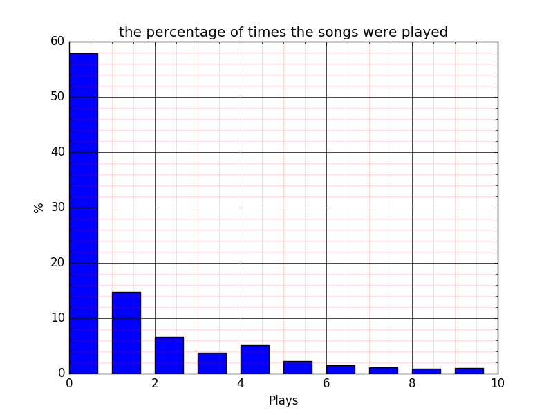
We note here about 58% of the songs were listened to only once.
Basic Recommender System
The most basic method is simply to recommend the most listened songs ! this method may seem obvious and too easy, but it actually works in many cases and to solve many problems like the cold start.
#!/usr/bin/env python
import graphlab as gl
import graphlab.aggregate as agg
import sqlite3

# Loading the DB
conn = sqlite3.connect("msd.sqlite3")

plays_df = gl.SFrame.from_sql(conn, "SELECT * FROM train")
songs_df = gl.SFrame.from_sql(conn, "SELECT * FROM song")

# Get the most listened songs
songs_total_listens = plays_df.groupby(key_columns='songID', operations={"plays": agg.SUM("plays")})

# Join songs with data
songs_total_listens = songs_total_listens.join(songs_df, on="songID", how="inner").sort("plays", ascending=False)
print "# Top Songs with most total lisens:"
print songs_total_listens.print_rows()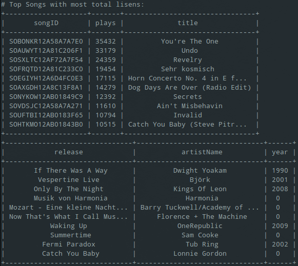
Similarity Recommendater
The principle is to base the similarity on the songs listened to by the user. Therefore two songs are considered similar if they were already listened to by the same user (which means the plays/ratings are ignored). There is many algorithms for item similarity like cosine, pearson and jaccard.
In the following code, we will use the Graphlab’s item similarity recommender (which uses jaccard by default) to calculate similarity, train the model, and calculate the RMSE.
#!/usr/bin/env python
import graphlab as gl
import sqlite3

# Load dataset
conn = sqlite3.connect("msd.sqlite3")
listens = gl.SFrame.from_sql(conn, "SELECT * FROM train")

# Create Training set and test set
train_data, test_data = gl.recommender.util.random_split_by_user(listens, "userID", "songID")

# Train the model
model = gl.item_similarity_recommender.create(train_data, "userID", "songID")

# Evaluate the model
rmse_data = model.evaluate_rmse(test_data, target="plays")

# Print the results
print rmse_data
We get an overall RMSE of 6.776336098094174
Factorization Recommander
In this category of recommendation algorithm, we have the choice between favoring “ranking performance” (predecting the order of the songs that a user will like) or “rating performance” (predicting the exact number of songs plays by a user).
Rating Performance :
In case we care mostly about rating performance, then we should use Factorization Recommender :
#!/usr/bin/env python
import sqlite3
import graphlab as gl

# Load datasets
conn = sqlite3.connect("msd.sqlite3")
listens = gl.SFrame.from_sql(conn, "SELECT * FROM train")

# Build model
training_data, validation_data = gl.recommender.util.random_split_by_user(listens, "userID", "songID")

# Train the model
model = gl.recommender.factorization_recommender.create(training_data, user_id="userID", item_id="songID", target="plays")

# Evaluate the model
rmse_data = model.evaluate_rmse(validation_data, target="plays")

# Print the results
print rmse_data
We get a little bit higher overall RMSE of 6.8547462552984095
Ranking Performance :
But If we care about ranking performance, then we should use Ranking Factorization Recommender instead :
#!/usr/bin/env python
import sqlite3
import graphlab as gl

# Load datasets
conn = sqlite3.connect("msd.sqlite3")
listens = gl.SFrame.from_sql(conn, "SELECT * FROM train")

# Build model
training_data, validation_data = gl.recommender.util.random_split_by_user(listens, "userID", "songID")

# Train the model
model = gl.recommender.ranking_factorization_recommender.create(training_data, user_id="userID", item_id="songID", target="plays")

# Recommend songs to users
rmse_data = model.evaluate_rmse(validation_data, target="plays")

# Print the results
print rmse_data
We get clearly a better overall RMSE of 8.342124685755607
Results & Optimization
Based on the analysis of the algorithms and the results, clearly, Ranking Factorization Recommender class model is the best suited for our database.
We note from the analysis we made at the beginning of the database that we can exclude listening to songs listened only once, and we assume that a single play of a song is not enough to take it into consideration:
#!/usr/bin/env python
import sqlite3
import graphlab as gl

# Load datasets
conn = sqlite3.connect("msd.sqlite3")
listens = gl.SFrame.from_sql(conn, "SELECT * FROM train where plays >=2")

# Build model
training_data, validation_data = gl.recommender.util.random_split_by_user(listens, "userID", "songID")

# Train the model
model = gl.recommender.ranking_factorization_recommender.create(training_data, user_id="userID", item_id="songID", target="plays")

# Evaluate the model
rmse_data = model.evaluate_rmse(validation_data, target="plays")

# Print the results
print rmse_data
Clearly, we get even better results with this optimization, the overall RMSE is 9.804972175313402
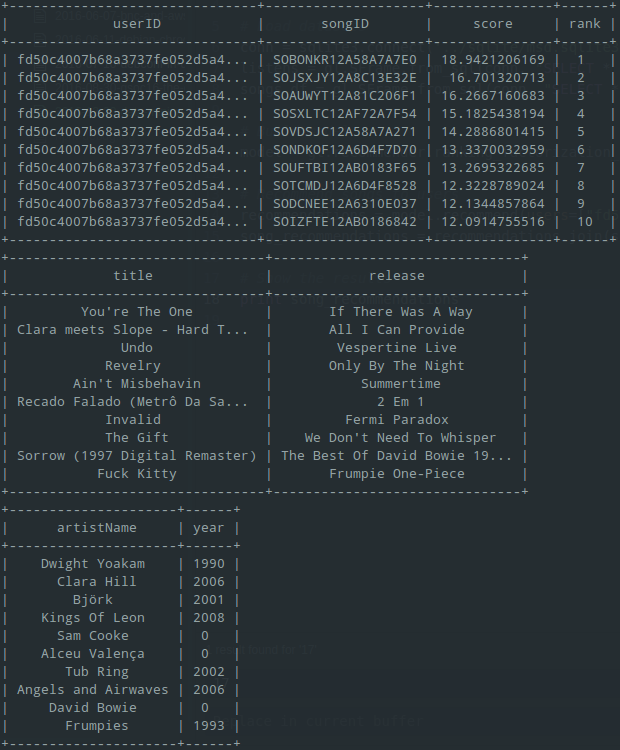
Recommend Songs
Let’s use an example user to see songs the model recommends for him:
#!/usr/bin/env python
import sqlite3
import graphlab as gl

# Load datasets
conn = sqlite3.connect("msd.sqlite3")
listens = gl.SFrame.from_sql(conn, "SELECT * FROM train where plays >=2")
songs_df = gl.SFrame.from_sql(conn, "SELECT * FROM song")

# Build model
model = gl.recommender.ranking_factorization_recommender.create(listens, user_id="userID", item_id="songID", target="plays")

# Recommend songs to users
recommendations = model.recommend(users=["fd50c4007b68a3737fe052d5a4f78ce8aa117f3d"])
song_recommendations = recommendations.join(songs_df, on="songID", how="inner").sort("rank")

# Show the results
print song_recommendations
TA DA ! we get songs recommendations as expected :
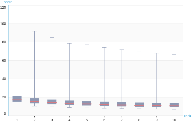
If we recommend songs for all the users, we will get the follow plot showing the distribution of calculated scores by rank :
Conclusion
Recommendations can be generated by a wide range of algorithms. While user-based or item-based collaborative filtering methods are simple and intuitive, matrix factorization techniques are usually more effective because they allow us to discover the latent features underlying the interactions between users and items.
Sources

Mouaad Aallam
Software Engineer